How does active learning reduce annotation costs?

Active learning reduces annotation costs by eliminating redundant labels. In a standard passive learning workflow, many labeled samples provide overlapping information the model already knows. Active learning uses query strategies like uncertainty sampling to identify only the samples that sit near the model decision boundary or represent underexplored regions of the feature space. Annotating fewer but more informative samples produces the same model quality at a fraction of the cost.

What is uncertainty sampling in active learning?

Uncertainty sampling is the most widely used active learning query strategy. The model scores each unlabeled sample by how uncertain it is about the correct label, and the samples with the highest uncertainty scores are selected for human annotation. Common uncertainty measures include prediction confidence (1 minus the probability of the top predicted class), margin sampling (the difference between the top two predicted probabilities), and entropy (the distribution of uncertainty across all classes).

What is the cold start problem in active learning?

The cold start problem occurs at the beginning of an active learning loop when no labeled data exists to train a model that can generate uncertainty scores. Without an initial model, there is no basis for selecting informative samples. The standard solutions are random seed selection (annotate 50 to 200 randomly chosen samples to bootstrap the first model), cluster-based initialization (select samples that represent the diversity of the unlabeled pool), and LLM-based pre-labeling (use a large language model to generate initial pseudo-labels that a human then reviews and corrects).

What is query by committee in active learning?

Query by committee is an active learning strategy that trains multiple models (the committee) on the same labeled set and selects samples where the committee members disagree most. High disagreement among committee members indicates that a sample carries information that would meaningfully update model weights. Query by committee tends to produce more diverse selected batches than uncertainty sampling from a single model.

When should I use active learning instead of labeling the full dataset?

Use active learning when your annotation budget is constrained, when your unlabeled dataset is large relative to what you can afford to label, when labeling is expensive due to domain expertise requirements such as medical, legal, or industrial data, or when you need to iterate rapidly on model quality. Active learning is most valuable when the unlabeled pool is at least 10 times larger than what you can afford to label.

How do I know when to stop an active learning loop?

Stop the active learning loop when model performance on your validation set plateaus across two or more consecutive annotation rounds, when the annotation budget is exhausted, or when labeled set coverage across all target classes reaches your quality threshold. Performance plateau means the marginal accuracy gain per annotation round has dropped below your minimum acceptable improvement threshold, typically 0.5 to 1 percent per round for mature models.

Does active learning work for computer vision annotation?

Yes. Active learning works well for computer vision tasks including image classification, object detection, and segmentation. Research published in the Springer Journal of Computational Social Science shows that annotating only 20 to 25 percent of total data achieves 95 percent of full-dataset performance on image classification tasks. For object detection and segmentation, annotation cost reductions of 40 to 60 percent are achievable in production settings.

Active Learning for Data Annotation: How to Label Less and Build Better Models

Annotation is the bottleneck for almost every machine learning project. Eighty percent of AI project time goes toward data preparation and labeling, and the global data annotation market is on track to grow from 4.87 billion dollars in 2025 to 29.11 billion dollars by 2032. Most of that cost is human time spent reviewing samples your model could have learned to handle on its own.

Active learning is the discipline of making your model ask for exactly the labels it needs rather than consuming labels indiscriminately. Applied correctly, it reduces annotation effort by 30 to 70 percent while preserving model accuracy. This guide covers every component of an active learning system: what it is, how query strategies work, how to solve the cold start problem, how to know when to stop, and what the benchmarks say about real-world results.

Quick Answer: What Is Active Learning in Data Annotation?

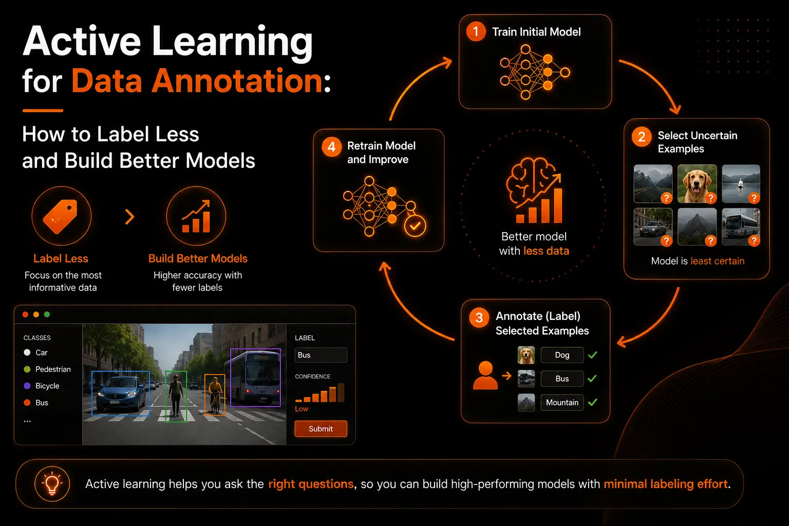
Active Learning for Data Annotation: How to Label Less and Build Better Models

Active learning is a machine learning strategy in which the model selects the specific unlabeled samples it most needs human labels for. Rather than annotating a dataset uniformly, you label only the samples that carry the most training value for the current model state. The loop runs iteratively: train, select, label, retrain.

Definition: the model asks for labels on the samples it is most uncertain about or finds most informative

Typical annotation reduction: 30 to 70 percent fewer labels required to reach the same model accuracy

Core components: unlabeled pool, query strategy, human annotator (oracle), labeled set, model

Best fit: large unlabeled datasets, expensive annotation domains, constrained labeling budgets

Not ideal for: tiny datasets, tasks where every sample is equally informative, projects requiring full ground-truth coverage

How the Active Learning Loop Works

The active learning loop is a structured cycle that replaces the one-shot annotation paradigm used in most standard machine learning projects. Instead of labeling everything and then training, you alternate between labeling and training in rounds.

The Five Stages of the Active Learning Loop

Understanding the loop stages is essential before choosing a query strategy or building a pipeline. Each stage has a defined input, output, and failure mode.

Stage 1 (Seed Set): select 50 to 200 samples at random, label them manually, and use them to train the first model; this provides the initial uncertainty estimates needed for Stage 2

Stage 2 (Query): apply your query strategy to score every sample in the unlabeled pool and select the top-ranked batch; batch size is typically 1 to 5 percent of the unlabeled pool per round

Stage 3 (Annotation): route the selected batch to human annotators; annotation time per round is the main cost driver and scales linearly with batch size

Stage 4 (Retraining): add newly labeled samples to the labeled set and retrain the model; track validation accuracy after each round to measure improvement

Stage 5 (Stopping Check): evaluate whether stopping criteria are met; if not, return to Stage 2 with the updated model

What Makes a Sample Informative

Informativeness is the key concept in active learning. A sample is informative if labeling it would cause the model to update its weights meaningfully. Samples that the model already classifies confidently contribute little new information and are deprioritized.Informative samples typically fall into three categories: samples near the decision boundary where the model probability output is close to equal across classes, samples from underrepresented regions of the feature space that the current training set does not cover, and samples that expose contradictions between multiple models trained on the same data.

Pool-Based vs Stream-Based Active Learning

Most production annotation workflows use pool-based active learning: you have a fixed pool of unlabeled samples and apply a query strategy to rank and select from that pool in batches. Stream-based active learning processes samples one at a time in a stream and decides in real time whether to request a label. Pool-based is more practical for annotation pipelines because it aligns with batch annotation workflows and allows the query strategy to consider global pool characteristics.

Five Query Strategies: How the Model Selects What to Label

The query strategy determines which unlabeled samples are selected for annotation in each round. Choosing the right strategy for your task and dataset structure is the most important decision in active learning system design.

Uncertainty Sampling

Uncertainty sampling is the most widely used active learning strategy. The model assigns a confidence score to each unlabeled sample and selects the samples with the lowest confidence for annotation. Three specific formulations define how uncertainty is measured.

Least confidence: select samples where the probability of the top predicted class is lowest; simplest to implement; works well for binary and low-class-count problems

Margin sampling: select samples where the margin between the top two predicted class probabilities is smallest; more informative than least confidence for multi-class problems

Entropy sampling: select samples with the highest entropy across the full predicted probability distribution; captures uncertainty across all classes simultaneously; best default choice for multi-class classification

Limitation: uncertainty sampling can oversample from outliers and mislabeled data; apply a confidence floor to exclude samples with corrupted features

Query by Committee

Query by committee trains an ensemble of models (the committee) on the same labeled set using different architectures, initializations, or random seeds. Samples where committee members disagree most are selected for annotation.The disagreement metric is typically vote entropy (how spread the predicted class votes are across committee members) or average KL-divergence between member probability distributions. Query by committee naturally produces diverse selected batches because disagreement reflects both boundary proximity and feature space coverage gaps.

Best for: tasks where a single model uncertainty estimate is noisy; use cases where diversity in selected batches matters more than pure boundary proximity

Committee size: 3 to 7 models is sufficient for most production workflows; larger committees increase computational cost without proportional accuracy gains

Limitation: training and maintaining multiple models increases infrastructure cost; batch-mode QBC (selecting top-k disagreement samples at once) is more practical than single-sample querying

Diversity Sampling and Core-Set Approaches

Diversity sampling selects samples that maximize coverage of the unlabeled feature space rather than targeting the model decision boundary. Core-set methods find the smallest subset of unlabeled samples that adequately represents the full unlabeled pool in the embedding space.Diversity sampling is most valuable during early annotation rounds when the labeled set is small and the model uncertainty estimates are unreliable. Combining diversity sampling in early rounds with uncertainty sampling in later rounds is a common production strategy.

K-means clustering: cluster the unlabeled pool and select representative samples from each cluster; ensures labeled set covers all discovered data clusters

Core-set (greedy): iteratively add the unlabeled sample that is furthest from any currently labeled sample in the embedding space; produces the most coverage-maximizing labeled set

Best for: early annotation rounds, cold start recovery, tasks with high visual or semantic diversity in the unlabeled pool

Expected Model Change and Expected Error Reduction

Expected model change selects samples that are predicted to cause the largest gradient update if labeled. Expected error reduction selects samples that are predicted to reduce the model generalization error the most if labeled. Both are more theoretically motivated than uncertainty or diversity sampling but are computationally expensive because they require forward passes for each candidate sample across all possible labels.

Expected gradient length (EGL): selects samples predicted to produce the largest gradient norm; scales well to deep learning but requires gradient computation per candidate

Expected error reduction: directly optimizes for generalization; computationally prohibitive for large unlabeled pools without approximation; practical primarily for small datasets

Use when: you have sufficient compute budget and want maximum theoretical annotation efficiency; often overkill for pools of more than 10,000 samples

Density-Weighted Sampling

Density-weighted sampling multiplies the informativeness score of each sample by its density in the feature space. This prevents uncertainty sampling from repeatedly selecting outliers (low-density, high-uncertainty samples that carry little generalizable information). The density weight ensures that selected samples are both uncertain and representative of the broader data distribution.

Formula: informativeness(x) = uncertainty(x) x density(x) where density is estimated by average similarity to other unlabeled samples in the pool

Benefit: reduces the impact of mislabeled or corrupted samples on the query selection process

Limitation: estimating density for high-dimensional data requires approximate methods; kernel density estimation or kNN average distance are the most practical approaches

The Cold Start Problem and Three Ways to Solve It

The cold start problem is the most common practical barrier to adopting active learning. It refers to the state at the beginning of a project when there are no labeled samples to train the initial model that generates uncertainty scores for the query strategy. Without a model, there is no uncertainty signal, and without an uncertainty signal, there is no basis for selecting informative samples.

Solution 1: Random Seed Selection

The simplest cold start solution is to select an initial labeled set at random and use it to bootstrap the first model. A random seed of 50 to 200 samples is sufficient for most tasks. The first round of active learning uses this bootstrap model, which is deliberately imperfect, to generate the first uncertainty-ranked batch for annotation.

Seed size guidance: 50 samples for binary classification, 100 to 200 for multi-class, 200 to 500 for object detection and segmentation tasks

Advantage: zero additional infrastructure required; straightforward to implement in any annotation platform

Limitation: random seeds provide no guarantee of class coverage; use stratified sampling if class labels are available for at least a portion of the pool

Solution 2: Cluster-Based Warm Start

Cluster-based warm start uses an unsupervised clustering algorithm to group the unlabeled pool by feature similarity, then selects representative samples from each cluster for the initial seed. This ensures that the seed set covers the diversity of the unlabeled pool rather than drawing from one cluster at random.

Implementation: embed all unlabeled samples using a pretrained feature extractor (ResNet, CLIP, or a sentence transformer), run k-means clustering, select one representative sample per cluster for annotation

Cluster count: use 5 to 10 clusters for the initial seed; more clusters require more annotation but provide better initialization

Advantage: eliminates the coverage risk of purely random seeds; the initial model trains on a sample that represents the full distribution

Solution 3: LLM-Based Pre-Labeling

A more recent approach uses a large language model or a foundation model (such as CLIP, GPT-4V, or Gemini) to generate pseudo-labels for the full unlabeled pool before any human annotation takes place. The active learning loop then starts with a large labeled set, but the initial labels are low-quality pseudo-labels that human annotators review and correct only where the LLM confidence is low.Research published in the Wiley International Journal of Intelligent Systems in 2025 shows that LLM-integrated active learning retains more than 93 percent of classification performance while requiring only about 6 percent of the computational time and cost of full manual labeling. This approach is particularly effective for text classification, image classification, and named entity recognition tasks where foundation models have strong zero-shot performance.

Pre-label with LLM at zero-shot or few-shot confidence thresholds

Accept LLM labels above the confidence threshold without human review (typically 0.85 to 0.95 predicted probability)

Route low-confidence samples to human annotators for review and correction

Train the initial model on accepted pseudo-labels plus human-reviewed corrections

Continue the standard active learning loop from this warm start position

Active Learning vs Semi-Supervised Learning vs Weak Supervision

Active learning is frequently confused with semi-supervised learning and weak supervision because all three reduce the number of human-annotated labels required to train a model. The distinctions matter for pipeline design and expected outcomes.

When to Choose Active Learning Over the Alternatives

Method	How It Reduces Annotation	Human Involvement	Label Quality	Best Use Case
Active Learning	Selects the most informative samples for human labeling; ignores the rest	High: human labels every selected sample	High: all accepted labels are human-verified	Large unlabeled pools with expensive per-label annotation costs
Semi-Supervised Learning	Trains on a small labeled set plus pseudo-labels generated for unlabeled data	Low: human labels only the initial seed set	Mixed: pseudo-labels introduce noise; quality degrades on hard samples	Tasks where the model can generalize well from a small seed; image classification
Weak Supervision	Uses labeling functions (heuristics, rules, distant supervision) to generate noisy labels at scale	Low to medium: human writes labeling functions rather than labels samples	Lower: labels are programmatically generated and inherently noisy	NLP tasks where labeling functions can be defined; document classification, relation extraction
Active Learning + Semi-Supervised (hybrid)	Uses active learning to select informative samples and semi-supervised learning to leverage unlabeled remainder	Medium: human labels active learning selections only	High on selected samples; mixed on pseudo-labeled remainder	Very large unlabeled pools where budget allows only 1 to 5 percent labeled data

Choose active learning when annotation quality must be high and every label is human-verified: medical imaging, legal document classification, safety-critical computer vision

Choose semi-supervised learning when your labeled seed set generalizes well and label noise on pseudo-labeled samples is acceptable: general image classification, sentiment analysis on broad domains

Choose weak supervision when you can write effective labeling functions and speed of label generation matters more than per-label accuracy: large-scale NLP, relation extraction, document routing

Use hybrid approaches when your unlabeled pool is very large (100,000 or more samples) and your budget allows labeling only 1 to 5 percent of the pool

How to Build an Active Learning Pipeline: Step-by-Step

A production active learning pipeline connects your annotation platform, model training infrastructure, and query strategy into a repeating loop. This section covers each component and how to connect them.

Step 1: Define the Annotation Schema and Quality Threshold

Before starting any annotation, define exactly what annotators should label, how edge cases are handled, and what inter-annotator agreement threshold is acceptable. Schema decisions made before the first seed round propagate through every subsequent round and cannot be easily changed once labeling begins.

Define all label classes with precise written definitions before labeling the seed set

Specify the minimum acceptable inter-annotator agreement (target Cohen's kappa of 0.8 or above for most tasks)

Document edge case handling rules for ambiguous samples that could be classified differently by different annotators

Establish the minimum labeled set size required to declare the project complete (the stopping target)

Step 2: Prepare and Embed the Unlabeled Pool

Embed all unlabeled samples using a pretrained feature extractor appropriate for your data modality. This embedding is used both for cluster-based warm start and for density-weighted query strategies. Computing embeddings upfront avoids repeated computation in later rounds.

Images: use ResNet-50, CLIP ViT-B/32, or EfficientNet embeddings; compute and store as numpy arrays

Text: use sentence-transformers (all-MiniLM-L6-v2 or similar) or GPT-4 embeddings; store as vector database for fast nearest-neighbor queries

Tabular data: use autoencoders or statistical feature normalization; PCA reduction to 50 to 100 dimensions is sufficient for most active learning query strategies

Step 3: Annotate the Seed Set

Label 50 to 200 samples using cluster-based selection or random selection. Upload labeled samples to your training pipeline. Train the first model checkpoint. This is the only round where no query strategy is applied.

Step 4: Run the Query Strategy and Select the Next Batch

Apply your chosen query strategy (uncertainty sampling, query by committee, or diversity sampling) to rank all remaining unlabeled samples. Select the top-ranked batch for annotation. Batch size should balance annotator throughput (smaller batches allow faster model updates) against infrastructure overhead (larger batches reduce retraining frequency).

Early rounds (low model confidence): use diversity sampling or cluster-based selection to maximize coverage; the model is not yet reliable enough for uncertainty estimates

Mid rounds (improving model): switch to uncertainty sampling (entropy or margin); the model now has meaningful decision boundary structure

Late rounds (mature model): use density-weighted uncertainty sampling to avoid over-sampling outliers near the boundary

Step 5: Annotate the Selected Batch

Route the selected batch to annotators. Apply the annotation schema defined in Step 1. Use your annotation platform's review workflow to flag samples that annotators disagree on or find ambiguous. Resolve disagreements before adding them to the labeled set. Do not include unresolved disagreements in the training data.

Step 6: Retrain and Evaluate

Add the newly labeled batch to the labeled set. Retrain the model from scratch or fine-tune from the previous checkpoint depending on the model architecture and batch size. Evaluate on the held-out validation set and record the accuracy or F1 score for this round. Plot the learning curve (accuracy vs labeled set size) to track efficiency over time.

Retrain from scratch for small models (fewer than 50 million parameters) where convergence is fast

Fine-tune from the previous checkpoint for large models where retraining from scratch is computationally prohibitive

Always evaluate on the same fixed validation set across all rounds so that performance comparisons are valid

What Active Learning Actually Delivers: Benchmarks and Results

Active learning works in theory. The question for production teams is whether the annotation reduction is large enough to justify the added pipeline complexity. The following benchmarks are drawn from peer-reviewed research published between 2024 and 2026.

Clinical NLP: Named Entity Recognition (PMC/JAMIA, July 2024)

A study published in the Journal of the American Medical Informatics Association tested five active learning strategies on clinical named entity recognition using a BioClinicalBERT model with pool-based annotation. Results showed that all five active learning strategies reduced the number of tokens that required human review compared to random sampling.

CLUSTER strategy: reduced token review by 19.3 percent vs random sampling at 98 percent target effectiveness

NBSE strategy: reduced token review by 59.2 percent vs random sampling at 98 percent target effectiveness

CNBSE strategy (the study best performer): required 20.4 percent fewer edits than NBSE and 22.5 percent fewer edits for challenging entities at 99 percent target effectiveness

At 98 percent effectiveness, the CLUSTER strategy achieved an average annotation rate of just 4.0 percent of total tokens, meaning human review was needed for only 1 in 25 tokens

Image Classification: Retail Product Recognition (Springer, 2024)

Research published in the Springer Journal of Computational Social Science evaluated active learning on retail product recognition, a task that requires high inter-class discrimination for thousands of product SKUs. Results showed that annotating only 20.83 to 24.34 percent of total data achieves 95 percent of the accuracy attainable with the full labeled dataset.

Text Classification: BERT-Based Models (Neural Computing and Applications, 2026)

A 2026 study in Springer Neural Computing and Applications found that active learning enables a 50 percent reduction in dataset size in 70 percent of text classification test cases using BERT-based models, without sacrificing model effectiveness metrics.

Medical Imaging: Ultrasound Datasets (ScienceDirect, 2024)

A cost-focused framework published in ScienceDirect demonstrated that manual annotation can be reduced by 66 percent using active learning on ultrasound datasets, with only a 4 percent accuracy drop from theoretical maximums achievable with full annotation.

LLM-Integrated Active Learning (Wiley, 2025)

Research published in the Wiley International Journal of Intelligent Systems in 2025 showed that LLM-integrated active learning retains more than 93 percent of classification performance while requiring only about 6 percent of the computational time and cost of fully supervised labeling with no active learning.

Stopping Criteria: When to End the Active Learning Loop

Knowing when to stop is as important as knowing how to start. Continuing annotation rounds past the point of diminishing returns wastes annotation budget without meaningful model improvement. Three stopping criteria cover the majority of production cases.

Criterion 1: Performance Plateau

Monitor validation set accuracy (or F1 score, mAP, or your task-specific metric) after each annotation round. If improvement across two or more consecutive rounds falls below a minimum acceptable threshold, the model has reached a performance plateau and additional annotation is unlikely to produce meaningful gains.

Set the minimum acceptable improvement threshold before the loop starts: 0.5 to 1 percent per round is a typical threshold for mature models with 1,000 or more labeled samples

Declare a plateau when two consecutive rounds both fall below the minimum improvement threshold

Do not adjust the threshold downward mid-project to justify continuing annotation; this defeats the purpose of the stopping criterion

Criterion 2: Budget Exhaustion

Set a maximum annotation budget at project start in terms of labeled sample count, annotation hours, or annotation cost. Stop when the budget is reached regardless of current model performance. If the model has not reached the target accuracy by budget exhaustion, the annotation budget, the task difficulty, or the quality of the unlabeled pool requires reassessment before additional labeling.

Criterion 3: Class Coverage Threshold

For tasks with multiple output classes, monitor labeled set coverage across all classes. If the active learning process has not produced sufficient labeled examples for rare classes (classes that appear infrequently in the unlabeled pool), the model will underperform on those classes regardless of aggregate accuracy. Continue annotation rounds focused on underrepresented classes until the coverage threshold is met.

Minimum per-class sample count: set a floor (e.g., 50 labeled samples per class minimum) before declaring the active learning loop complete

Use stratified sampling to supplement active learning selection when rare classes are consistently under-selected by the query strategy

Track per-class F1 score alongside aggregate accuracy to detect class-level performance gaps before stopping

Criterion 4: Confidence Distribution Shift

As the active learning loop progresses, the distribution of model confidence scores on the unlabeled pool should shift toward higher confidence (lower uncertainty). When the pool-wide average uncertainty drops below a threshold indicating that the model is confident about nearly all remaining unlabeled samples, continuing annotation provides diminishing returns regardless of absolute performance.

Active Learning for Computer Vision, NLP, and Medical Imaging

Active learning strategies perform differently across data modalities because the sources of informativeness and the cost of annotation vary significantly. This section covers the practical differences for the three most common annotation domains.

Computer Vision: Image Classification and Object Detection

For image classification, uncertainty sampling with entropy scoring is the standard baseline query strategy. CLIP or ResNet embeddings provide the feature space for diversity sampling during early rounds. For object detection, active learning at the image level (selecting which images to annotate) is more practical than sample-level selection because annotation cost is driven by image count rather than object count.

Image classification: entropy-based uncertainty sampling; target is 20 to 25 percent of the pool to reach 95 percent of full-dataset accuracy

Object detection: select images with the highest aggregate uncertainty across predicted bounding boxes; YOLO and Faster R-CNN both provide per-box confidence scores

Semantic segmentation: select images with the highest spatial uncertainty (pixel-level entropy averaged across the image); note that annotation time per image is high regardless of AL selection

Natural Language Processing: Text Classification and NER

For text classification, uncertainty sampling with margin or entropy scoring is highly effective because pre-trained transformer models (BERT, RoBERTa) provide calibrated probability estimates. For named entity recognition, token-level uncertainty is aggregated to the sentence level to determine which sentences require annotation.

Text classification: margin sampling identifies the sentences closest to the decision boundary; effective for sentiment analysis, topic classification, intent detection

NER: token-level entropy aggregated by sentence (average entropy per token); target the 4 to 6 percent of tokens shown in clinical NER research to require review at 98 percent effectiveness

Use LLM pre-labeling to address the cold start problem in NLP tasks; GPT-4 and Claude zero-shot labels are high quality on broad-domain classification and NER

Medical Imaging: High-Cost, High-Stakes Annotation

Medical imaging annotation is the highest-value use case for active learning because per-sample annotation cost is high (requiring clinical expertise), the unlabeled pool is often large (hospital PACS systems contain millions of images), and model performance targets are extremely demanding. The annotation reduction from active learning has direct economic and operational impact.

Target tasks: radiology report generation, pathology slide classification, ultrasound structure detection, dermatology image classification

Research shows 66 percent manual annotation reduction on ultrasound datasets with only 4 percent accuracy drop (ScienceDirect, 2024)

Clinical NER showed annotation rates as low as 4 percent of total tokens required at 98 percent effectiveness (PMC JAMIA, 2024)

Combine active learning with calibrated uncertainty (temperature scaling or conformal prediction) to ensure uncertainty scores are reliable for clinical safety requirements

When Active Learning Is Not the Right Choice

Active learning adds pipeline complexity: you need query strategy infrastructure, round-based annotation workflows, and retraining between rounds. For some projects, that complexity is not justified by the annotation savings.

Cases Where Active Learning Provides Minimal Value

Small datasets: if your total unlabeled pool is fewer than 500 samples, the overhead of an active learning loop exceeds the savings; label everything manually

Uniformly informative data: if all samples in the pool are roughly equally informative (e.g., every sample is a unique, novel image), uncertainty sampling will select near-randomly anyway

Short annotation timelines: if the project requires a fully labeled dataset within days, the round-based annotation structure of active learning may extend the timeline compared to parallel full-pool annotation

Full ground truth required: some downstream applications (regulatory compliance, benchmark dataset creation, legal document review) require every sample to be labeled regardless of model performance; active learning does not apply

Annotation cost is very low: if annotators can label thousands of samples per hour with low cost per label (e.g., binary sentiment labels on Twitter data), the savings from active learning may not justify the pipeline complexity

Failure Modes to Avoid

Active learning can underperform passive labeling when the query strategy consistently selects outliers and mislabeled samples that have high uncertainty but low generalizable information. This problem is addressed by density-weighted sampling and by setting a minimum pool density threshold below which samples are excluded from selection regardless of uncertainty score.

Outlier selection bias: uncertainty sampling selects boundary-adjacent samples, which can include corrupted or atypical data; apply density weighting to reduce this effect

Class imbalance amplification: if rare classes are also low-uncertainty (few samples for the model to be uncertain about), active learning may systematically under-select them; add a per-class selection constraint

Label drift: if annotation guidelines evolve between rounds, early and late round labels may be inconsistent; lock the annotation schema before starting the loop

Start Using Active Learning with Scematics

Scematics provides annotation workflows designed for iterative active learning pipelines. The platform supports round-based batch annotation, inter-annotator agreement tracking, multi-format export for retraining integration, and managed annotation services staffed by domain-expert annotators.If you are evaluating active learning for a specific project, the Scematics team can review your unlabeled pool characteristics, annotation budget, and model accuracy targets to recommend a query strategy and pipeline configuration aligned with your requirements. Self-serve platform access and fully managed annotation services are both available.

Scematics Copyrights Reserved